TCP的报文结构(TCP segment structure)
basic structure
Interactive applications,however, often transmit data chunks that are smaller than the MSS; for example, with remote login applications like Telnet, the data field in the TCP segment is often only one byte. Because the TCP header is typically 20 bytes (12 bytes more than the UDP header), segments sent by Telnet may be only 21 bytes in length. Figure bellow shows the structure of the TCP segment.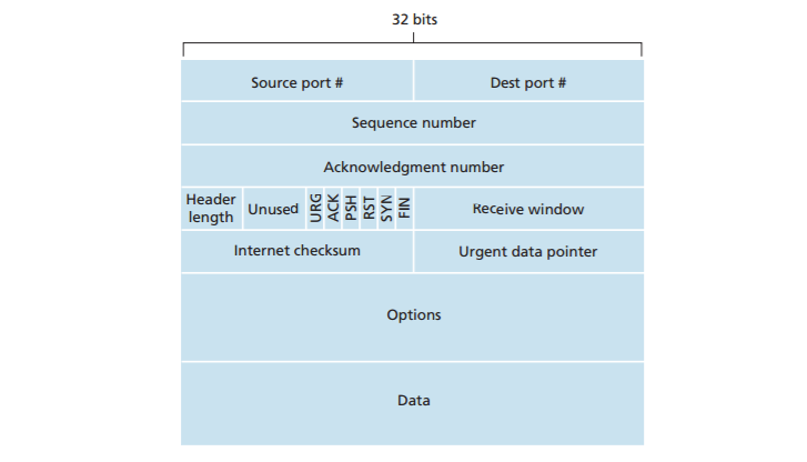
As with UDP, the header includes source and destination port numbers , which are used for multiplexing/demultiplexing data from/to upper-layer applications. Also, as with UDP, the header includes a checksum field . A TCP segment header also contains the following fields:
- The 32-bit sequence number field and the 32-bit acknowledgment number field are used by the TCP sender and receiver in implementing a reliable data transfer service, as discussed below.
- The 16-bit receive window field is used for flow control. We will see shortly that it is used to indicate the number of bytes that a receiver is willing to accept.
- The 4-bit header length field specifies the length of the TCP header in 32-bit words. The TCP header can be of variable length due to the TCP options field.
- The optional and variable-length options field is used when a sender and receiver negotiate the maximum segment size (MSS) or as a window scaling factor for use in high-speed networks. A time-stamping option is also defined. See RFC 854 and RFC 1323 for additional details.
- The flag field contains 6 bits. The ACK bit is used to indicate that the value carried in the acknowledgment field is valid; that is, the segment contains an acknowledgment for a segment that has been successfully received. The RST, SYN, and FIN bits are used for connection setup and teardown, as we will discuss at the end of this section. Setting the PSH bit indicates that the receiver should pass the data to the upper layer immediately. Finally, the URG bit is used to indicate that there is data in this segment that the sending-side upper-layer entity has marked as “urgent.” The location of the last byte of this urgent data is indicated by the 16-bit urgent data pointer field. TCP must inform the receiving-side upper-layer entity when urgent data exists and pass it a pointer to the end of the urgent data. (In practice, the PSH, URG, and the urgent data pointer are not used. However, we mention these fields for completeness.)
Demo: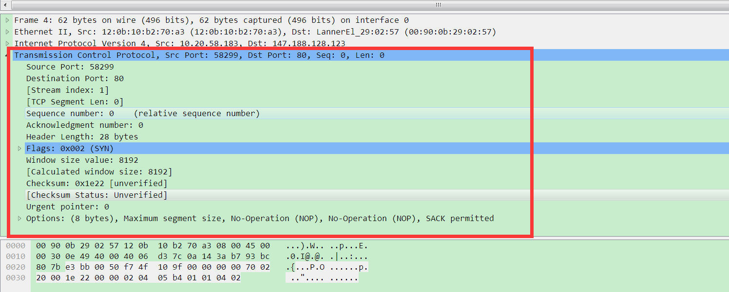
Sequence Numbers and Acknowledgment Numbers
Two of the most important fields in the TCP segment header are the sequence number field and the acknowledgment number field. These fields are a critical part of TCP’s reliable data transfer service. But before discussing how these fields are used to provide reliable data transfer, let us first explain what exactly TCP puts in these fields.
TCP views data as an unstructured, but ordered, stream of bytes. TCP’s use of sequence numbers reflects this view in that sequence numbers are over the stream of transmitted bytes and not over the series of transmitted segments. The sequence number for a segment is therefore the byte-stream number of the first byte in the segment. Let’s look at an example. Suppose that a process in Host A wants to send a stream of data to a process in Host B over a TCP connection. The TCP in Host A will implicitly number each byte in the data stream. Suppose that the data stream consists of a file consisting of 500,000 bytes, that the MSS is 1,000 bytes, and that the first byte of the data stream is numbered 0.As shown in Figure bellow,
TCP constructs 500 segments out of the data stream. The first segment gets assigned sequence number 0, the second segment gets assigned sequence number 1,000, the third segment gets assigned sequence number 2,000, and so on. Each sequence number is inserted in the sequence number field in the header of the appropriate TCP segment.
Now let’s consider acknowledgment numbers. These are a little trickier than sequence numbers. Recall that TCP is full-duplex, so that Host A may be receiving data from Host B while it sends data to Host B (as part of the same TCP connection). Each of the segments that arrive from Host B has a sequence number for the data
flowing from B to A. The acknowledgment number that Host A puts in its segment is the sequence number of the next byte Host A is expecting from Host B. It is good to look at a few examples to understand what is going on here. Suppose that Host A has received all bytes numbered 0 through 535 from B and suppose that it is about
to send a segment to Host B. Host A is waiting for byte 536 and all the subsequent bytes in Host B’s data stream. So Host A puts 536 in the acknowledgment number field of the segment it sends to B.
As another example, suppose that Host A has received one segment from Host B containing bytes 0 through 535 and another segment containing bytes 900 through 1,000. For some reason Host A has not yet received bytes 536 through 899. In this example, Host A is still waiting for byte 536 (and beyond) in order to re-create B’s
data stream. Thus, A’s next segment to B will contain 536 in the acknowledgment number field. Because TCP only acknowledges bytes up to the first missing byte in the stream, TCP is said to provide cumulative acknowledgments.
This last example also brings up an important but subtle issue. Host A received the third segment (bytes 900 through 1,000) before receiving the second segment(bytes 536 through 899). Thus, the third segment arrived out of order. The subtle issue is: What does a host do when it receives out-of-order segments in a TCP connection?
Interestingly, the TCP RFCs do not impose any rules here and leave the decision up to the people programming a TCP implementation. There are basically two choices: either (1) the receiver immediately discards out-of-order segments (which, as we discussed earlier, can simplify receiver design), or (2) the receiver keeps the out-of-order bytes and waits for the missing bytes to fill in the gaps. Clearly, the latter choice is more efficient in terms of network bandwidth, and is the approach taken in practice.
In Figure up, we assumed that the initial sequence number was zero. In truth,both sides of a TCP connection randomly choose an initial sequence number. This is done to minimize the possibility that a segment that is still present in the network from an earlier, already-terminated connection between two hosts is mistaken for a
valid segment in a later connection between these same two hosts (which also happen to be using the same port numbers as the old connection) [Sunshine 1978].Telnet: A Case Study for Sequence and Acknowledgment Numbers
Telnet, defined in RFC 854, is a popular application-layer protocol used for remote login. It runs over TCP and is designed to work between any pair of hosts. Unlike the bulk data transfer applications discussed in Chapter 2, Telnet is an interactive application. We discuss a Telnet example here, as it nicely illustrates TCP sequence and acknowledgment numbers. We note that many users now prefer to use the SSH protocol rather than Telnet, since data sent in a Telnet connection (including passwords!) is not encrypted, making Telnet vulnerable to eavesdropping attacks
Suppose Host A initiates a Telnet session with Host B. Because Host A initiates the session, it is labeled the client, and Host B is labeled the server. Each character typed by the user (at the client) will be sent to the remote host; the remote host will send back a copy of each character, which will be displayed on the Telnet user’s screen. This “echo back” is used to ensure that characters seen by the Telnet user have already been received and processed at the remote site. Each character thus traverses the network twice between the time the user hits the key and the time the character is displayed on the user’s monitor
Now suppose the user types a single letter, ‘C,’and then grabs a coffee. Let’s examine the TCP segments that are sent between the client and server. As shown in Figure 3.31, we suppose the starting sequence numbers are 42 and 79 for the client and server, respectively.Recall that the sequence number of a segment is the sequence number of the first byte in the data field. Thus, the first segment sent from the client will have sequence number 42; the first segment sent from the server will have sequence number Recall that the acknowledgment number is the sequence number of the next byte of data that the host is waiting for. After the TCP connection is established but before any data is sent, the client is waiting for byte 79 and the server is waiting for byte 42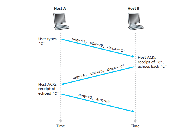
As shown in Figure 3.31, three segments are sent. The first segment is sent from the client to the server, containing the 1-byte ASCII representation of the letter ‘C’ in its data field. This first segment also has 42 in its sequence number field, as we just described. Also, because the client has not yet received any data from the server, this first segment will have 79 in its acknowledgment number field
The second segment is sent from the server to the client. It serves a dual purpose.First it provides an acknowledgment of the data the server has received. By putting 43 in the acknowledgment field, the server is telling the client that it has successfully received everything up through byte 42 and is now waiting for bytes 43 onward. The second purpose of this segment is to echo back the letter ‘C.’ Thus, the second segment has the ASCII representation of ‘C’ in its data field. This second segment has the sequence number 79, the initial sequence number of the server-toclient data flow of this TCP connection, as this is the very first byte of data that the server is sending. Note that the acknowledgment for client-to-server data is carried in a segment carrying server-to-client data; this acknowledgment is said to be piggybacked on the server-to-client data segmentRound-Trip Time Estimation and Timeout
TCP, like our rdt protocol in Section 3.4, uses a timeout/retransmit mechanism to recover from lost segments. Although this is conceptually simple, many subtle issues arise when we implement a timeout/retransmit mechanism in an actual protocol such as TCP. Perhaps the most obvious question is the length of the timeout
intervals. Clearly, the timeout should be larger than the connection’s round-trip time (RTT), that is, the time from when a segment is sent until it is acknowledged. Otherwise, unnecessary retransmissions would be sent. But how much larger? How should the RTT be estimated in the first place? Should a timer be associated with each and every unacknowledged segment? So many questions! Our discussion in this section is based on the TCP work in [Jacobson 1988] and the current IETF recommendations for managing TCP timers [RFC 6298].Estimating the Round-Trip Time
Let’s begin our study of TCP timer management by considering how TCP estimates the round-trip time between sender and receiver. This is accomplished as follows. The sample RTT, denoted SampleRTT, for a segment is the amount of time between when the segment is sent (that is, passed to IP) and when an acknowledgment for the segment is received. Instead of measuring a SampleRTT for every transmitted segment, most TCP implementations take only one SampleRTT measurement at a time. That is, at any point in time, the SampleRTT is being estimated
for only one of the transmitted but currently unacknowledged segments, leading to a new value of SampleRTT approximately once every RTT. Also, TCP never computes a SampleRTT for a segment that has been retransmitted; it only measures SampleRTT for segments that have been transmitted once [Karn 1987]. (A problem at the end of the chapter asks you to consider why.)
Obviously, the SampleRTT values will fluctuate from segment to segment due to congestion in the routers and to the varying load on the end systems. Because of this fluctuation, any given SampleRTT value may be atypical. In order to estimate a typical RTT, it is therefore natural to take some sort of average of the SampleRTT
values. TCP maintains an average, called EstimatedRTT, of the SampleRTT values. Upon obtaining a new SampleRTT, TCP updates EstimatedRTT according to the following formula:
$$EstimatedRTT = (1 – a) • EstimatedRTT + a• SampleRTT$$
The formula above is written in the form of a programming-language statement—the new value of EstimatedRTT is a weighted combination of the previous value of EstimatedRTT and the new value for SampleRTT. The recommended value of is = 0.125 (that is, 1/8) [RFC 6298], in which case the formula above becomes:
$$EstimatedRTT = 0.875 • EstimatedRTT + 0.125 • SampleRTT$$Setting and Managing the Retransmission Timeout Interval
Given values of EstimatedRTT and DevRTT, what value should be used for TCP’s timeout interval? Clearly, the interval should be greater than or equal to EstimatedRTT, or unnecessary retransmissions would be sent. But the timeout interval should not be too much larger than EstimatedRTT; otherwise, when a segment is lost, TCP would not quickly retransmit the segment, leading to large data transfer delays. It is therefore desirable to set the timeout equal to the EstimatedRTT plus some margin. The margin should be large when there is a lot of fluctuation in the SampleRTT values; it should be small when there is little fluctuation. The value of
DevRTT should thus come into play here. All of these considerations are taken into account in TCP’s method for determining the retransmission timeout interval:
$$TimeoutInterval = EstimatedRTT + 4 • DevRTT$$
An initial TimeoutInterval value of 1 second is recommended [RFC 6298].Also, when a timeout occurs, the value of TimeoutInterval is doubled to avoid a premature timeout occurring for a subsequent segment that will soon be acknowledged.However, as soon as a segment is received and EstimatedRTT is updated,
the TimeoutInterval is again computed using the formula above.Reliable Data Transfer
Recall that the Internet’s network-layer service (IP service) is unreliable. IP does not guarantee datagram delivery, does not guarantee in-order delivery of datagrams, and does not guarantee the integrity of the data in the datagrams. With IP service, datagrams can overflow router buffers and never reach their destination,
datagrams can arrive out of order, and bits in the datagram can get corrupted(flipped from 0 to 1 and vice versa). Because transport-layer segments are carried across the network by IP datagrams, transport-layer segments can suffer from these problems as well TCP creates a reliable data transfer service on top of IP’s unreliable besteffort service. TCP’s reliable data transfer service ensures that the data stream that a process reads out of its TCP receive buffer is uncorrupted, without gaps, without duplication, and in sequence; that is, the byte stream is exactly the same byte stream that was sent by the end system on the other side of the connection. How TCP provides a reliable data transfer involves many of the principles that we studied in Section 3.4 In our earlier development of reliable data transfer techniques, it was conceptually easiest to assume that an individual timer is associated with each transmitted but not yet acknowledged segment. While this is great in theory, timer management can require considerable overhead. Thus, the recommended TCP timer management procedures [RFC 6298] use only a single retransmission timer, even if there are multiple transmitted but not yet acknowledged segments. The TCP protocol described in this section follows this single-timer recommendation
We will discuss how TCP provides reliable data transfer in two incremental steps. We first present a highly simplified description of a TCP sender that uses only timeouts to recover from lost segments; we then present a more complete description that uses duplicate acknowledgments in addition to timeouts. In the ensuing discussion, we suppose that data is being sent in only one direction, from Host A to Host B, and that Host A is sending a large file
Figure 3.33 presents a highly simplified description of a TCP sender. We see that there are three major events related to data transmission and retransmission in the TCP sender: data received from application above; timer timeout; and ACK receipt. Upon the occurrence of the first major event, TCP receives data from the application, encapsulates the data in a segment, and passes the segment to IP. Note that each segment includes a sequence number that is the byte-stream number of the first data byte in the segment, as described in Section 3.5.2. Also note that if the timer is already not running for some other segment, TCP starts the timer when the segment is passed to IP. (It is helpful to think of the timer as being associated with the oldest unacknowledged segment.) The expiration interval for this timer is the TimeoutInterval, which is calculated from EstimatedRTT and DevRTT, as described in Section 3.5.3.
The second major event is the timeout. TCP responds to the timeout event by retransmitting the segment that caused the timeout. TCP then restarts the timer
The third major event that must be handled by the TCP sender is the arrival of an acknowledgment segment (ACK) from the receiver (more specifically, a segment containing a valid ACK field value). On the occurrence of this event, TCP compares the ACK value y with its variable SendBase. The TCP state variable SendBase is the sequence number of the oldest unacknowledged byte. (Thus SendBase–1 is the sequence number of the last byte that is known to have been received correctly and in order at the receiver.) As indicated earlier, TCP uses cumulative acknowledgments, so that y acknowledges the receipt of all bytes before byte number y. If y > SendBase, then the ACK is acknowledging one or more previously unacknowledged segments.Thus the sender updates its SendBase variable; it also restarts the timer if there currently are any not-yet-acknowledged segments.A Few Interesting Scenarios
We have just described a highly simplified version of how TCP provides reliable data transfer. But even this highly simplified version has many subtleties. To get a good feeling for how this protocol works, let’s now walk through a few simple scenarios.
Figure 3.34 depicts the first scenario, in which Host A sends one segment to Host B. Suppose that this segment has sequence number 92 and contains 8 bytes of data. After sending this segment, Host A waits for a segment from B with acknowledgment number 100. Although the segment from A is received at B, the acknowledgment from B to A gets lost. In this case, the timeout event occurs, and Host A retransmits the same segment. Of course, when Host B receives the retransmission, it observes from the sequence number that the segment contains
data that has already been received. Thus, TCP in Host B will discard the bytes in the retransmitted segment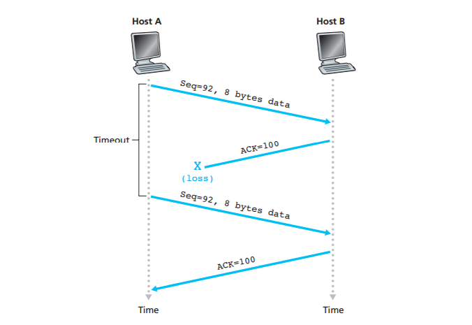
In a second scenario, shown in Figure 3.35, Host A sends two segments back to back. The first segment has sequence number 92 and 8 bytes of data, and the second segment has sequence number 100 and 20 bytes of data. Suppose that both segments arrive intact at B, and B sends two separate acknowledgments for each of these segments. The first of these acknowledgments has acknowledgment number 100; the second has acknowledgment number 120. Suppose now that neither of the acknowledgments arrives at Host A before the timeout. When the timeout event occurs, Host A resends the first segment with sequence number 92 and restarts the timer. As long
as the ACK for the second segment arrives before the new timeout, the second segment will not be retransmitted
In a third and final scenario, suppose Host A sends the two segments, exactly as in the second example. The acknowledgment of the first segment is lost in the network, but just before the timeout event, Host A receives an acknowledgment with acknowledgment number 120. Host A therefore knows that Host B has received everything up through byte 119; so Host A does not resend either of the two segments. This scenario is illustrated in Figure
Doubling the Timeout Interval
We now discuss a few modifications that most TCP implementations employ. The first concerns the length of the timeout interval after a timer expiration. In this modification, whenever the timeout event occurs, TCP retransmits the not-yetacknowledged segment with the smallest sequence number, as described above. But
each time TCP retransmits, it sets the next timeout interval to twice the previous value, rather than deriving it from the last EstimatedRTT and DevRTT (as described in Section 3.5.3). For example, suppose TimeoutInterval associated with the oldest not yet acknowledged segment is .75 sec when the timer first expires.TCP will then retransmit this segment and set the new expiration time to 1.5 sec. If the timer expires again 1.5 sec later, TCP will again retransmit this segment, now setting the expiration time to 3.0 sec. Thus the intervals grow exponentially after each retransmission. However, whenever the timer is started after either of the two other events (that is, data received from application above, and ACK received), the TimeoutInterval is derived from the most recent values of EstimatedRTT and DevRTT.
This modification provides a limited form of congestion control. (More comprehensive forms of TCP congestion control will be studied in Section 3.7.) The timer expiration is most likely caused by congestion in the network, that is, too many packets arriving at one (or more) router queues in the path between the source
and destination, causing packets to be dropped and/or long queuing delays. In times of congestion, if the sources continue to retransmit packets persistently, the congestion may get worse. Instead, TCP acts more politely, with each sender retransmitting after longer and longer intervals. We will see that a similar idea is used by Ethernet when we study CSMA/CD in Chapter 5
Fast Retransmit
One of the problems with timeout-triggered retransmissions is that the timeout period can be relatively long. When a segment is lost, this long timeout period forces the sender to delay resending the lost packet, thereby increasing the end-to end delay. Fortunately, the sender can often detect packet loss well before the timeout
event occurs by noting so-called duplicate ACKs. A duplicate ACK is an ACK that reacknowledges a segment for which the sender has already received an earlier acknowledgment. To understand the sender’s response to a duplicate ACK, we must look at why the receiver sends a duplicate ACK in the first place. Table 3.2 summarizes the TCP receiver’s ACK generation policy [RFC 5681]. When a TCP receiver receives a segment with a sequence number that is larger than the next, expected,in-order sequence number, it detects a gap in the data stream—that is, a missing segment.This gap could be the result of lost or reordered segments within the network.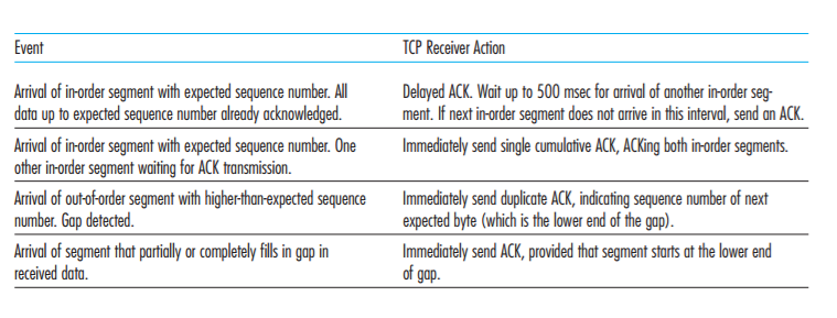
Since TCP does not use negative acknowledgments, the receiver cannot send an explicit negative acknowledgment back to the sender. Instead, it simply reacknowledges (that is, generates a duplicate ACK for) the last in-order byte of data it has received. (Note that Table 3.2 allows for the case that the receiver does not discard
out-of-order segments.) Because a sender often sends a large number of segments back to back, if one segment
is lost, there will likely be many back-to-back duplicate ACKs. If the TCP sender receives three duplicate ACKs for the same data, it takes this as an indication that the segment following the segment that has been ACKed three times has been lost. (In the homework problems, we consider the question of why the sender waits for three duplicate ACKs, rather than just a single duplicate ACK.) In the case that three duplicate ACKs are received, the TCP sender performs a fast retransmit [RFC 5681], retransmitting the missing segment before that segment’s timer expires. This is shown in Figure 3.37, where the second segment is lost, then retransmitted before its timer expires. For TCP with fast retransmit, the following code snippet replaces the ACK received event in Figure 3.33: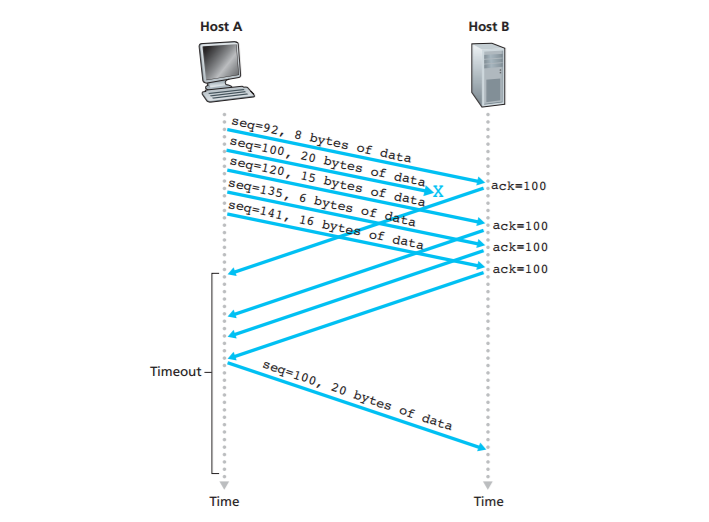
We noted earlier that many subtle issues arise when a timeout/retransmit mechanism is implemented in an actual protocol such as TCP. The procedures above,which have evolved as a result of more than 20 years of experience with TCP timers, should convince you that this is indeed the case!
Go-Back-N or Selective Repeat?
Let us close our study of TCP’s error-recovery mechanism by considering the following question: Is TCP a GBN or an SR protocol? Recall that TCP acknowledgments are cumulative and correctly received but out-of-order segments are not individually
ACKed by the receiver. Consequently, as shown in Figure 3.33 (see also Figure 3.19),the TCP sender need only maintain the smallest sequence number of a transmitted but unacknowledged byte (SendBase) and the sequence number of the next byte to be sent (NextSeqNum). In this sense, TCP looks a lot like a GBN-style protocol. But
there are some striking differences between TCP and Go-Back-N. Many TCP implementations will buffer correctly received but out-of-order segments [Stevens 1994]. Consider also what happens when the sender sends a sequence of segments 1, 2, . . . , N, and all of the segments arrive in order without error at the receiver. Further suppose that the acknowledgment for packet n < N gets lost, but the remaining N – 1 acknowledgments
arrive at the sender before their respective timeouts. In this example, GBN would retransmit not only packet n, but also all of the subsequent packets n + 1, n + 2,. . . , N. TCP, on the other hand, would retransmit at most one segment, namely, segment n. Moreover, TCP would not even retransmit segment n if the acknowledgment for segment n + 1 arrived before the timeout for segment n.
A proposed modification to TCP, the so-called selective acknowledgment [RFC 2018], allows a TCP receiver to acknowledge out-of-order segments selectively rather than just cumulatively acknowledging the last correctly received, inorder segment. When combined with selective retransmission—skipping the retransmission of segments that have already been selectively acknowledged by the receiver—TCP looks a lot like our generic SR protocol. Thus, TCP’s error-recovery mechanism is probably best categorized as a hybrid of GBN and SR protocols.
Flow Control
Recall that the hosts on each side of a TCP connection set aside a receive buffer for the connection. When the TCP connection receives bytes that are correct and in sequence, it places the data in the receive buffer. The associated application process will read data from this buffer, but not necessarily at the instant the data arrives.Indeed, the receiving application may be busy with some other task and may not even attempt to read the data until long after it has arrived. If the application is relatively slow at reading the data, the sender can very easily overflow the connection’s receive buffer by sending too much data too quickly
TCP provides a flow-control service to its applications to eliminate the possibility of the sender overflowing the receiver’s buffer. Flow control is thus a speed-matching service—matching the rate at which the sender is sending against the rate at which the receiving application is reading. As noted earlier, a TCP sender can also be throttled due to congestion within the IP network; this form of sender control is referred to as congestion control, a topic we will explore in detail in Sections 3.6 and 3.7. Even though the actions taken by flow and congestion control are similar (the throttling of the sender), they are obviously taken for very different reasons. Unfortunately, many authors use the terms interchangeably, and the savvy reader would be wise to distinguish between them. Let’s now discuss how TCP provides its flow-control service. In order to see the forest for the trees, we suppose throughout this section that the TCP implementation is such that the TCP receiver discards out-of-order segments
TCP provides flow control by having the sender maintain a variable called the receive window. Informally, the receive window is used to give the sender an idea of how much free buffer space is available at the receiver. Because TCP is full-duplex, the sender at each side of the connection maintains a distinct receive window. Let’s investigate the receive window in the context of a file transfer. Suppose that Host A is sending
a large file to Host B over a TCP connection. Host B allocates a receive buffer to this connection; denote its size by RcvBuffer. From time to time, the application process in Host B reads from the buffer. Define the following variables:
- LastByteRead: the number of the last byte in the data stream read from the
buffer by the application process in B - LastByteRcvd: the number of the last byte in the data stream that has arrived
from the network and has been placed in the receive buffer at B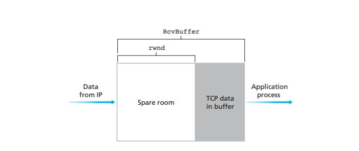
Because TCP is not permitted to overflow the allocated buffer, we must have
$$LastByteRcvd – LastByteRead <= RcvBuffer$$
The receive window, denoted rwnd is set to the amount of spare room in the buffer:
$$rwnd = RcvBuffer – [LastByteRcvd – LastByteRead]$$
Because the spare room changes with time, rwnd is dynamic. The variable rwnd is
illustrated in Figure 3
Host A in turn keeps track of two variables, LastByteSent and LastByteAcked, which have obvious meanings. Note that the difference between these two variables, LastByteSent – LastByteAcked, is the amount of unacknowledged
data that A has sent into the connection. By keeping the amount of unacknowledged data less than the value of rwnd, Host A is assured that it is not overflowing the receive buffer at Host B. Thus, Host A makes sure throughout the connection’s life that
$$LastByteSent – LastByteAcked <= rwnd$$
There is one minor technical problem with this scheme. To see this, suppose Host B’s receive buffer becomes full so that rwnd = 0. After advertising rwnd = 0 to Host A, also suppose that B has nothing to send to A. Now consider what happens. As the application process at B empties the buffer, TCP does not send new segments
with new rwnd values to Host A; indeed, TCP sends a segment to Host A only if it has data to send or if it has an acknowledgment to send. Therefore, Host A is never informed that some space has opened up in Host B’s receive buffer—Host A is blocked and can transmit no more data! To solve this problem, the TCP specification
requires Host A to continue to send segments with one data byte when B’s receive window is zero. These segments will be acknowledged by the receiver. Eventually the buffer will begin to empty and the acknowledgments will contain a nonzero rwnd value
The online site at http://www.awl.com/kurose-ross for this book provides an interactive Java applet that illustrates the operation of the TCP receive window. Having described TCP’s flow-control service, we briefly mention here that UDP does not provide flow control. To understand the issue, consider sending a series of UDP segments from a process on Host A to a process on Host B. For a typical UDP implementation, UDP will append the segments in a finite-sized buffer that “precedes” the corresponding socket (that is, the door to the process). The process reads one entire segment at a time from the buffer. If the process does not read the segments fast enough from the buffer, the buffer will overflow and segments will get dropped.
TCP Connection Management
In this subsection we take a closer look at how a TCP connection is established and torn down. Although this topic may not seem particularly thrilling, it is important because TCP connection establishment can significantly add to perceived delays (for example, when surfing the Web). Furthermore, many of the most common network attacks—including the incredibly popular SYN flood attack—exploit vulnerabilities in TCP connection management.
Open a TCP connection
Let’s first take a look at how a TCP connection is established. Suppose a process running in one host (client) wants to initiate a connection with another process in another host (server). The client application process first informs the client TCP that it wants to establish a connection to a process in the server. The TCP in the client then proceeds to establish a TCP connection with the TCP in the server in the following manner:
- Step 1. The client-side TCP first sends a special TCP segment to the server-side TCP. This special segment contains no application-layer data. But one of the flag bits in the segment’s header (see Figure 3.29), the SYN bit, is set to 1. For this reason, this special segment is referred to as a SYN segment. In addition, the client randomly chooses an initial sequence number (client_isn) and puts this number in the sequence number field of the initial TCP SYN segment. This segment is encapsulated within an IP datagram and sent to the server. There has been considerable interest in properly randomizing the choice of the client_isn in order to avoid certain security attacks [CERT 2001–09].
- Step 2. Once the IP datagram containing the TCP SYN segment arrives at the server host (assuming it does arrive!), the server extracts the TCP SYN segment from the datagram, allocates the TCP buffers and variables to the connection, and sends a connection-granted segment to the client TCP. (We’ll see in Chapter 8 that
the allocation of these buffers and variables before completing the third step of the three-way handshake makes TCP vulnerable to a denial-of-service attack known as SYN flooding.) This connection-granted segment also contains no applicationlayer data. However, it does contain three important pieces of information in the
segment header. First, the SYN bit is set to 1. Second, the acknowledgment field of the TCP segment header is set to client_isn+1. Finally, the server chooses its own initial sequence number (server_isn) and puts this value in the sequence number field of the TCP segment header. This connection-granted segment is saying, in effect, “I received your SYN packet to start a connection with your initial sequence number, client_isn. I agree to establish this connection. My own initial sequence number is server_isn.” The connectiongranted segment is referred to as a SYNACK segment. - Step 3. Upon receiving the SYNACK segment, the client also allocates buffers and variables to the connection. The client host then sends the server yet another segment; this last segment acknowledges the server’s connection-granted segment (the client does so by putting the value server_isn+1 in the acknowledgment
field of the TCP segment header). The SYN bit is set to zero, since the connection is established. This third stage of the three-way handshake may carry client-to-server data in the segment payload.
Once these three steps have been completed, the client and server hosts can send segments containing data to each other. In each of these future segments, the SYN bit will be set to zero. Note that in order to establish the connection, three packets are sent between the two hosts, as illustrated in Figure 3.39. For this reason, this connectionestablishment procedure is often referred to as a three-way handshake. Several aspects of the TCP three-way handshake are explored in the homework problems(Why are initial sequence numbers needed? Why is a three-way handshake, as opposed to a two-way handshake, needed?). It’s interesting to note that a rock climber
and a belayer (who is stationed below the rock climber and whose job it is to handle the climber’s safety rope) use a three-way-handshake communication protocol that is identical to TCP’s to ensure that both sides are ready before the climber begins ascent.
Close a TCP connection
All good things must come to an end, and the same is true with a TCP connection.Either of the two processes participating in a TCP connection can end the connection.When a connection ends, the “resources” (that is, the buffers and variables) in the hosts are deallocated. As an example, suppose the client decides to close the
connection, as shown in Figure 3.40. The client application process issues a close command. This causes the client TCP to send a special TCP segment to the server process. This special segment has a flag bit in the segment’s header, the FIN bit (see Figure 3.29), set to 1. When the server receives this segment, it sends the client an acknowledgment segment in return. The server then sends its own shutdown segment, which has the FIN bit set to 1. Finally, the client acknowledges the server’s shutdown segment. At this point, all the resources in the two hosts are now deallocated
During the life of a TCP connection, the TCP protocol running in each host makes transitions through various TCP states. Figure 3.41 illustrates a typical sequence of TCP states that are visited by the client TCP. The client TCP begins in the CLOSED state. The application on the client side initiates a new TCP connection
(by creating a Socket object in our Java examples as in the Python examples from Chapter 2). This causes TCP in the client to send a SYN segment to TCP in the server. After having sent the SYN segment, the client TCP enters the SYN_SENT state. While in the SYN_SENT state, the client TCP waits for a segment from the server TCP that includes an acknowledgment for the client’s previous segment and has the SYN bit set to 1. Having received such a segment, the client TCP enters the ESTABLISHED state. While in the ESTABLISHED state, the TCP client can send
and receive TCP segments containing payload (that is, application-generated) data
Principles of Congestion Control
In the previous sections, we examined both the general principles and specific TCP mechanisms used to provide for a reliable data transfer service in the face of packet loss. We mentioned earlier that, in practice, such loss typically results from the overflowing of router buffers as the network becomes congested. Packet
retransmission thus treats a symptom of network congestion (the loss of a specific transport-layer segment) but does not treat the cause of network congestion—too many sources attempting to send data at too high a rate. To treat the cause of network congestion, mechanisms are needed to throttle senders in the face of network
congestion.
In this section, we consider the problem of congestion control in a general context, seeking to understand why congestion is a bad thing, how network congestion is manifested in the performance received by upper-layer applications, and various approaches that can be taken to avoid, or react to, network congestion. This more
general study of congestion control is appropriate since, as with reliable data transfer, it is high on our “top-ten” list of fundamentally important problems in networking. We conclude this section with a discussion of congestion control in the available bit-rate (ABR) service in asynchronous transfer mode (ATM) networks. The following section contains a detailed study of TCP’s congestioncontrol algorithm.
The Causes and the Costs of Congestion
Let’s begin our general study of congestion control by examining three increasingly complex scenarios in which congestion occurs. In each case, we’ll look at why congestion occurs in the first place and at the cost of congestion (in terms of resources not fully utilized and poor performance received by the end systems). We’ll not (yet) focus on how to react to, or avoid, congestion but rather focus on the simpler issue of understanding what happens as hosts increase their transmission rate and the network becomes congested.
Scenario 1: Two Senders, a Router with Infinite Buffers
We begin by considering perhaps the simplest congestion scenario possible: Two hosts (A and B) each have a connection that shares a single hop between source and destination, as shown in Figure 3.43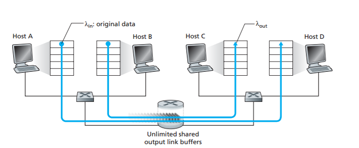
Let’s assume that the application in Host A is sending data into the connection (for example, passing data to the transport-level protocol via a socket) at an average rate of A_in bytes/sec. These data are original in the sense that each unit of data is sent into the socket only once. The underlying transport-level protocol is a simple one. Data is encapsulated and sent; no error recovery (for example, retransmission), flow control, or congestion control is performed. Ignoring the additional overhead due to adding transport- and lower-layer header information, the rate at which Host A offers traffic to the router in this first scenario is thus A_in bytes/sec. Host B operates in a similar manner, and we assume for simplicity that it too is sending at a rate of A_in bytes/sec. Packets from Hosts A and B pass through a router and over a shared outgoing link of capacity R. The router has buffers that allow it to store incoming packets when the packet-arrival rate exceeds the outgoing link’s capacity. In this first scenario, we assume that the router has an infinite amount of buffer space.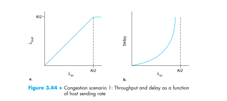
Figure 3.44 plots the performance of Host A’s connection under this first scenario. The left graph plots the per-connection throughput (number of bytes per second at the receiver) as a function of the connection-sending rate. For a sending rate between 0 and R/2, the throughput at the receiver equals the sender’s sending rate—everything sent by the sender is received at the receiver with a finite delay. When the sending rate is above R/2, however, the throughput is only R/2. This upper limit on throughput is a consequence of the sharing of link capacity between two connections. The link simply cannot deliver packets to a receiver at a steady-state
rate that exceeds R/2. No matter how high Hosts A and B set their sending rates, they will each never see a throughput higher than R/2.
Achieving a per-connection throughput of R/2 might actually appear to be a good thing, because the link is fully utilized in delivering packets to their destinations. The right-hand graph in Figure 3.44, however, shows the consequence of operating near link capacity. As the sending rate approaches R/2 (from the left), the average delay becomes larger and larger. When the sending rate exceeds R/2, the average number of queued packets in the router is unbounded, and the average delay between source and destination becomes infinite (assuming that the connections operate at these sending rates for an infinite period of time and there is an infinite amount of buffering available). Thus, while operating at an aggregate throughput of near R may be ideal from a throughput standpoint, it is far from ideal from a delay standpoint. Even in this (extremely) idealized scenario, we’ve already found one cost of a congested network—large queuing delays are experienced as the packetarrival rate nears the link capacity
Scenario 2: Two Senders and a Router with Finite Buffers
Let us now slightly modify scenario 1 in the following two ways (see Figure 3.45). First, the amount of router buffering is assumed to be finite. A consequence of this real-world assumption is that packets will be dropped when arriving to an already full buffer. Second, we assume that each connection is reliable. If a packet containing a transport-level segment is dropped at the router, the sender will eventually retransmit it. Because packets can be retransmitted, we must now be more careful with our use of the term sending rate. Specifically, let us again denote the rate at which the application sends original data into the socket by$ \lambda{in} $bytes/sec. The rate at which the transport layer sends segments (containing original data and retransmitted data) into the network will be denoted $\lambda1{in} $in bytes/sec. $\lambda1_{in} $ is sometimes referred to as the offered load to the network.
The performance realized under scenario 2 will now depend strongly on how retransmission is performed. First, consider the unrealistic case that Host A is able to somehow (magically!) determine whether or not a buffer is free in the router and thus sends a packet only when a buffer is free. In this case, no loss would occur,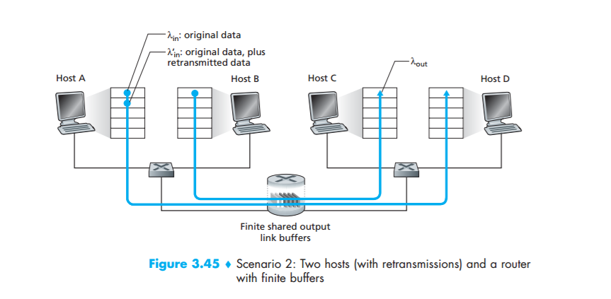
$\lambda1{in}$ would be equal to $\lambda{in}$, and the throughput of the connection would be equal to
$\lambda_{in}$. This case is shown in Figure 3.46(a). From a throughput standpoint, performance is ideal—everything that is sent is received. Note that the average host sending rate cannot exceed R/2 under this scenario, since packet loss is assumed never to occur.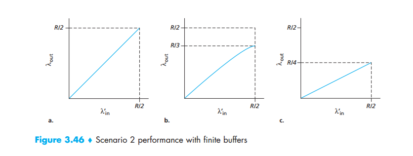
Consider next the slightly more realistic case that the sender retransmits only when a packet is known for certain to be lost. (Again, this assumption is a bit of a stretch. However, it is possible that the sending host might set its timeout large enough to be virtually assured that a packet that has not been acknowledged has been lost.) In this case, the performance might look something like that shown in Figure 3.46(b). To appreciate what is happening here, consider the case that the offered load, $\lambda1_{in}$ (the rate of original data transmission plus retransmissions), equals R/2. According to Figure 3.46(b), at this value of the offered load, the rate at which data are delivered to the receiver application is R/3. Thus, out of the 0.5R units of data transmitted, 0.333R bytes/sec (on average) are original data and 0.166R bytes/ sec (on average) are retransmitted data. We see here another cost of a congested network the sender must perform retransmissions in order to compensate for dropped (lost) packets due to buffer overflow
Finally, let us consider the case that the sender may time out prematurely and retransmit a packet that has been delayed in the queue but not yet lost. In this case, both the original data packet and the retransmission may reach the receiver. Of course, the receiver needs but one copy of this packet and will discard the retransmission. In this case, the work done by the router in forwarding the retransmitted copy of the original packet was wasted, as the receiver will have already received the original copy of this packet. The router would have better used the link transmission capacity to send a different packet instead. Here then is yet another cost of a congested network—unneeded retransmissions by the sender in the face of large delays may cause a router to use its link bandwidth to forward unneeded copies of a packet. Figure 3.46 (c) shows the throughput versus offered load when each packet is assumed to be forwarded (on average) twice by the router. Since each packet is forwarded twice, the throughput will have an asymptotic value of R/4 as the offered load approaches R/2.
Scenario 3: Four Senders, Routers with Finite Buffers, and Multihop Paths
In our final congestion scenario, four hosts transmit packets, each over overlapping two hop paths, as shown in Figure 3.47. We again assume that each host uses a timeout/retransmission mechanism to implement a reliable data transfer service, that all hosts have the same value of $\lambda_{in}$, and that all router links have capacity R bytes/sec.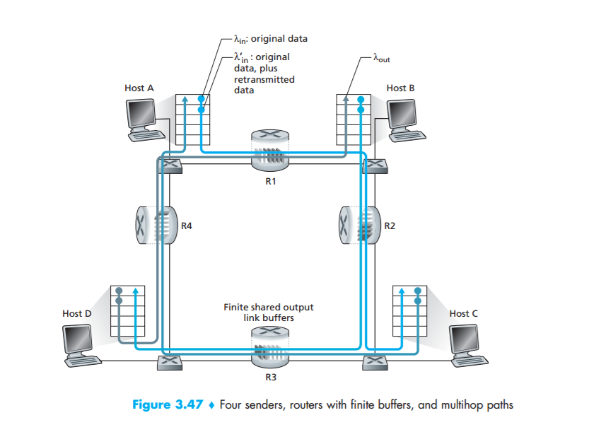
Let’s consider the connection from Host A to Host C, passing through routers R1 and R2. The A–C connection shares router R1 with the D–B connection and shares router R2 with the B–D connection. For extremely small values of $\lambda{in}$, buffer overflows are rare (as in congestion scenarios 1 and 2), and the throughput approximately equals the offered load. For slightly larger values of $\lambda{in}$, the corresponding throughput is also larger, since more original data is being transmitted into the network and delivered to the destination, and overflows are still rare. Thus, for small values of $\lambda{in}$, an increase in $\lambda1{in}$ results in an increase in $\lambda{out}$
Having considered the case of extremely low traffic, let’s next examine the case that $\lambda{in}$ (and hence $\lambda{in}$) is extremely large. Consider router R2. The A–C traffic arriving to router R2 (which arrives at R2 after being forwarded from R1) can have an arrival rate at R2 that is at most R, the capacity of the link from R1 to R2, regardless of the value of $\lambda{in}$. If $\lambda1_{in}$ is extremely large for all connections (including the B–D connection), then the arrival rate of B–D traffic at R2 can be much larger than that of the A–C traffic. Because the A–C and B–D traffic must compete at router R2 for the limited amount of buffer space, the amount of A–C traffic that successfully gets through R2 (that is, is not lost due to buffer overflow) becomes smaller and smaller as the offered load from B–D gets larger and larger. In the limit, as the offered load approaches infinity, an empty buffer at R2 is immediately filled by a B–D packet, and the throughput of the A–C connection at R2 goes to zero. This, in turn, implies that the A–C end-to-end throughput goes to zero in the limit of heavy traffic. These considerations give rise to the offered load versus throughput tradeoff shown in Figure 3.48.
The reason for the eventual decrease in throughput with increasing offered load is evident when one considers the amount of wasted work done by the network.In the high-traffic scenario outlined above, whenever a packet is dropped at a second-hop router, the work done by the first-hop router in forwarding a packet to the second-hop router ends up being “wasted.” The network would have been equally well off (more accurately, equally bad off) if the first router had simply discarded that packet and remained idle. More to the point, the transmission
capacity used at the first router to forward the packet to the second router could have been much more profitably used to transmit a different packet. (For example, when selecting a packet for transmission, it might be better for a router to give priority to packets that have already traversed some number of upstream
routers.)
TCP Congestion Control
In Section 3.7, we’ll examine TCP’s specific approach to congestion control in great detail. Here, we identify the two broad approaches to congestion control that are taken in practice and discuss specific network architectures and congestion-control protocols embodying these approaches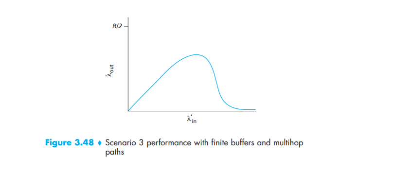
At the broadest level, we can distinguish among congestion-control approaches by whether the network layer provides any explicit assistance to the transport layer for congestion-control purposes:
End-to-end congestion control. In an end-to-end approach to congestion control, the network layer provides no explicit support to the transport layer for congestion control purposes. Even the presence of congestion in the network must be inferred by the end systems based only on observed network behavior (for example, packet
loss and delay). We will see in Section 3.7 that TCP must necessarily take this end to-end approach toward congestion control, since the IP layer provides no feedback to the end systems regarding network congestion. TCP segment loss (as indicated by a timeout or a triple duplicate acknowledgment) is taken as an indication of network congestion and TCP decreases its window size accordingly. We will also see a more recent proposal for TCP congestion control that uses increasing round-trip delay values as indicators of increased network congestion
CI and NI bits. As noted above, sender-to-receiver RM cells are interspersed with data cells. The rate of RM cell interspersion is a tunable parameter, with the default value being one RM cell every 32 data cells. These RM cells have a congestion indication (CI) bit and a no increase (NI) bit that can be set by a congested network switch. Specifically, a switch can set the NI bit in a passing RM cell to 1 under mild congestion and can set the CI bit to 1 under severe congestion conditions. When a destination host receives an RM cell, it will send the RM cell back to the sender with its CI and NI bits intact (except that CI may be set to 1 by the destination as a result of the EFCI mechanism described above).
ER setting. Each RM cell also contains a 2-byte explicit rate (ER) field. A congested switch may lower the value contained in the ER field in a passing RM cell. In this manner, the ER field will be set to the minimum supportable rate of all switches on the source-to-destination path.
TCP Congestion Control
In this section we return to our study of TCP. As we learned in Section 3.5, TCP provides a reliable transport service between two processes running on different hosts. Another key component of TCP is its congestion-control mechanism. As indicated in the previous section, TCP must use end-to-end congestion control rather than network-assisted congestion control, since the IP layer provides no explicit feedback to the end systems regarding network congestion
The approach taken by TCP is to have each sender limit the rate at which it sends traffic into its connection as a function of perceived network congestion. If a TCP sender perceives that there is little congestion on the path between itself and the destination, then the TCP sender increases its send rate; if the sender perceives
that there is congestion along the path, then the sender reduces its send rate. But this approach raises three questions. First, how does a TCP sender limit the rate at which it sends traffic into its connection? Second, how does a TCP sender perceive that there is congestion on the path between itself and the destination? And third, what algorithm should the sender use to change its send rate as a function of perceived end-to-end congestion?
Let’s first examine how a TCP sender limits the rate at which it sends traffic into its connection. In Section 3.5 we saw that each side of a TCP connection consists of a receive buffer, a send buffer, and several variables (LastByteRead, rwnd, and so on). The TCP congestion-control mechanism operating at the sender keeps
track of an additional variable, the congestion window. The congestion window, denoted cwnd, imposes a constraint on the rate at which a TCP sender can send traffic into the network. Specifically, the amount of unacknowledged data at a sender may not exceed the minimum of cwnd and rwnd, that is:
$$LastByteSent – LastByteAcked <= min{cwnd, rwnd}$$
In order to focus on congestion control (as opposed to flow control), let us henceforth assume that the TCP receive buffer is so large that the receive-window constraint can be ignored; thus, the amount of unacknowledged data at the sender is solely limited by cwnd. We will also assume that the sender always has data to send, i.e., that all segments in the congestion window are sent.
The constraint above limits the amount of unacknowledged data at the sender and therefore indirectly limits the sender’s send rate. To see this, consider a connection for which loss and packet transmission delays are negligible. Then, roughly, at the beginning of every RTT, the constraint permits the sender to send cwnd bytes of data into the connection; at the end of the RTT the sender receives acknowledgments for the data. Thus the sender’s send rate is roughly cwnd/RTT bytes/sec. By adjusting the value of cwnd, the sender can therefore adjust the rate at which it sends data into its connection
Let’s next consider how a TCP sender perceives that there is congestion on the path between itself and the destination. Let us define a “loss event” at a TCP sender as the occurrence of either a timeout or the receipt of three duplicate ACKs from the receiver. (Recall our discussion in Section 3.5.4 of the timeout event in Figure 3.33 and the subsequent modification to include fast retransmit on receipt of three duplicate ACKs.) When there is excessive congestion, then one (or more) router buffers along the path overflows, causing a datagram (containing a TCP segment) to be dropped. The dropped datagram, in turn, results in a loss event at the sender—either a timeout or the receipt of three duplicate ACKs—which is taken by the sender to be an indication of congestion on the sender-to-receiver path.
Having considered how congestion is detected, let’s next consider the more optimistic case when the network is congestion-free, that is, when a loss event doesn’t occur. In this case, acknowledgments for previously unacknowledged segments will be received at the TCP sender. As we’ll see, TCP will take the arrival of these acknowledgments as an indication that all is well—that segments being transmitted into the network are being successfully delivered to the destination—and will use acknowledgments to increase its congestion window
size (and hence its transmission rate). Note that if acknowledgments arrive at a relatively slow rate (e.g., if the end-end path has high delay or contains a low-bandwidth link), then the congestion window will be increased at a relatively slow rate. On the other hand, if acknowledgments arrive at a high rate, then the congestion window will be increased more quickly. Because TCP uses acknowledgments to trigger (or clock) its increase in congestion window size, TCP is said to be self-clocking
Given the mechanism of adjusting the value of cwnd to control the sending rate, the critical question remains: How should a TCP sender determine the rate at which it should send? If TCP senders collectively send too fast, they can congest the network,leading to the type of congestion collapse that we saw in Figure 3.48. Indeed,
the version of TCP that we’ll study shortly was developed in response to observed Internet congestion collapse [Jacobson 1988] under earlier versions of TCP. However, if TCP senders are too cautious and send too slowly, they could under utilize the bandwidth in the network; that is, the TCP senders could send at a higher rate
without congesting the network. How then do the TCP senders determine their sending rates such that they don’t congest the network but at the same time make use of all the available bandwidth? Are TCP senders explicitly coordinated, or is there a distributed approach in which the TCP senders can set their sending rates based only
on local information? TCP answers these questions using the following guiding principles:
- A lost segment implies congestion, and hence, the TCP sender’s rate should be decreased when a segment is lost. Recall from our discussion in Section 3.5.4, that a timeout event or the receipt of four acknowledgments for a given segment (one original ACK and then three duplicate ACKs) is interpreted as an implicit “loss event” indication of the segment following the quadruply ACKed segment, triggering a retransmission of the lost segment. From a congestioncontrol standpoint, the question is how the TCP sender should decrease its congestion
window size, and hence its sending rate, in response to this inferred loss event. - An acknowledged segment indicates that the network is delivering the sender’s segments to the receiver, and hence, the sender’s rate can be increased when an ACK arrives for a previously unacknowledged segment. The arrival of acknowledgments is taken as an implicit indication that all is well—segments are being successfully delivered from sender to receiver, and the network is thus not congested. The congestion window size can thus be increased.
- Bandwidth probing. Given ACKs indicating a congestion-free source-to-destination path and loss events indicating a congested path, TCP’s strategy for adjusting its transmission rate is to increase its rate in response to arriving ACKs until a loss event occurs, at which point, the transmission rate is decreased. The TCP sender thus increases its transmission rate to probe for the rate that at which congestion onset begins, backs off from that rate, and then to begins probing again to see if he congestion onset rate has changed. The TCP sender’s behavior is perhaps analogous to the child who requests (and gets) more and more goodies until finally he/she is finally told “No!”, backs off a bit, but then begins making requests again shortly afterwards. Note that there is no explicit signaling of congestion state by the network—ACKs and loss events serve as implicit signals—and that each TCP sender acts on local information asynchronously from other TCP
senders.
Given this overview of TCP congestion control, we’re now in a position to consider the details of the celebrated TCP congestion-control algorithm, which was first described in [Jacobson 1988] and is standardized in [RFC 5681]. The algorithm has three major components: (1) slow start, (2) congestion avoidance, and (3) fast recovery. Slow start and congestion avoidance are mandatory components of TCP, differing in how they increase the size of cwnd in response to received ACKs. We’ll see shortly that slow start increases the size of cwnd more rapidly (despite its name!) than congestion avoidance. Fast recovery is recommended, but not required, for
TCP senders.Slow Start
When a TCP connection begins, the value of cwnd is typically initialized to a small value of 1 MSS [RFC 3390], resulting in an initial sending rate of roughly MSS/RTT. For example, if MSS = 500 bytes and RTT = 200 msec, the resulting initial sending rate is only about 20 kbps. Since the available bandwidth to the TCP sender may be much larger than MSS/RTT, the TCP sender would like to find the amount of available bandwidth quickly. Thus, in the slow-start state, the value of cwnd begins at 1 MSS and increases by 1 MSS every time a transmitted
segment is first acknowledged. In the example of Figure 3.51, TCP sends the first segment into the network and waits for an acknowledgment. When this acknowledgment arrives, the TCP sender increases the congestion window by one MSS and sends out two maximum-sized segments. These segments are then acknowledged, with the sender increasing the congestion window by 1 MSS for each of the acknowledged segments, giving a congestion window of 4 MSS, and so on. This process results in a doubling of the sending rate every RTT. Thus, the TCP send rate starts slow but grows exponentially during the slow start phase.
But when should this exponential growth end? Slow start provides several answers to this question. First, if there is a loss event (i.e., congestion) indicated by a timeout, the TCP sender sets the value of cwnd to 1 and begins the slow start process anew. It also sets the value of a second state variable, ssthresh (shorthand for “slow start threshold”) to cwnd/2—half of the value of the congestion window value when congestion was detected. The second way in which slow start may end is directly tied to the value of ssthresh. Since ssthresh is half the value of cwnd when congestion was last detected, it might be a bit reckless to keep doubling cwnd when it reaches or surpasses the value of ssthresh. Thus, when the value of cwnd equals ssthresh, slow start ends and TCP transitions into congestion avoidance mode. As we’ll see, TCP increases
引用
《计算机网络-自顶向下方法(原书第五版)》